Tempeh Tech

Pre-Processing Effect

By Noël Jung

---

Content

1. Intro
2. Imports
3. Code
4. Conclusion

Intro

The most cumbersome step in producing chickpea tempeh for me is peeling and splitting the chickpeas. In earlier fermentations, I have not done that, as I had acceptable results without it. Lately, however, I am wondering whether this pre-processing would produce even better tempeh. Here, I do a side-by-side comparison. I produce two tempehs: One from peeled and split chickpeas, one without these steps, like I used to before. They go into the incubator at the same time, and I record the tempeh temperatures, to see how it behaves.

Imports

Import and data loading as seen previously.

import pandas as pd
import matplotlib as mpl
import matplotlib.pyplot as plt
import graph_style # Contains styling parameters for the plots.
from project_utils import time_parser, add_time_columns

EX_ID = "GC1"
CSV_FILE = rf"../CSV/{EX_ID}.csv"
ferm_data = pd.read_csv(CSV_FILE, parse_dates=["Time"], date_parser=time_parser)

# Transform time column into a readable format.
ferm_data["Time"] = ferm_data["Time"].dt.strftime("%d%m%Y-%H:%M:%S")
ferm_data = add_time_columns(ferm_data, new_columns=["h_passed", "min_passed"])

ferm_data.head()

	Time	name_dev_1	T_dev_1	name_dev_2	T_dev_2	T_CPU	min_passed	h_passed
0	10012024-20:49:36	28-3c01f09505ec	19.312	28-3c01f0953253	19.375	44.3	0	0
1	10012024-20:59:37	28-3c01f09505ec	19.937	28-3c01f0953253	19.75	41.8	10	0
2	10012024-21:09:39	28-3c01f09505ec	21.437	28-3c01f0953253	20.75	39.4	20	0
3	10012024-21:19:40	28-3c01f09505ec	23.0	28-3c01f0953253	21.937	40.4	30	1
4	10012024-21:29:42	28-3c01f09505ec	24.125	28-3c01f0953253	22.937	39.4	40	1

# Convert all values that are "failure" to None.
ferm_data["T_dev_1"] = ferm_data["T_dev_1"].replace("failure", None)
ferm_data["T_dev_2"] = ferm_data["T_dev_2"].replace("failure", None)

# Convert T_dev_1, and T_dev_2 to float.
ferm_data["T_dev_1"] = ferm_data["T_dev_1"].astype(float)
ferm_data["T_dev_2"] = ferm_data["T_dev_2"].astype(float)

Code

Let's plot the temperature curves.

# Save some variables for repeated use.
first_time = ferm_data["min_passed"].min() / 60
last_time = ferm_data["min_passed"].max() / 60

# Overwrite matplotlib default rcParams with custom styles.
for param, value in mpl.rcParamsDefault.items():
    mpl.rcParams[param] = graph_style.style.get(param, value)
mpl.rcParams["figure.figsize"] = (10, 4)
mpl.rcParams["font.family"] = graph_style.FONT

# Initialize temperature graphs.
fig, ax = plt.subplots()
ax.plot(ferm_data['min_passed']/60, ferm_data['T_dev_1'],
    label='T_dev_1', **graph_style.lineplot_kwargs, color=graph_style.colors_pomegranate[1])
ax.plot(ferm_data['min_passed']/60, ferm_data['T_dev_2'],
    label='T_dev_2', **graph_style.lineplot_kwargs, color=graph_style.colors_pomegranate_var[1])

# Add legend.
handles, labels = ax.get_legend_handles_labels()
legend_title = ax.legend(title=None, handles=handles,
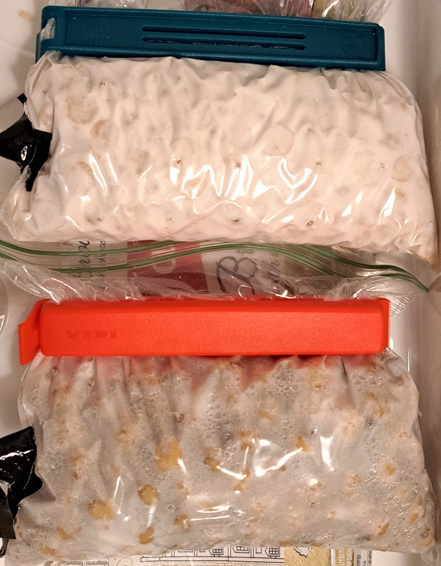
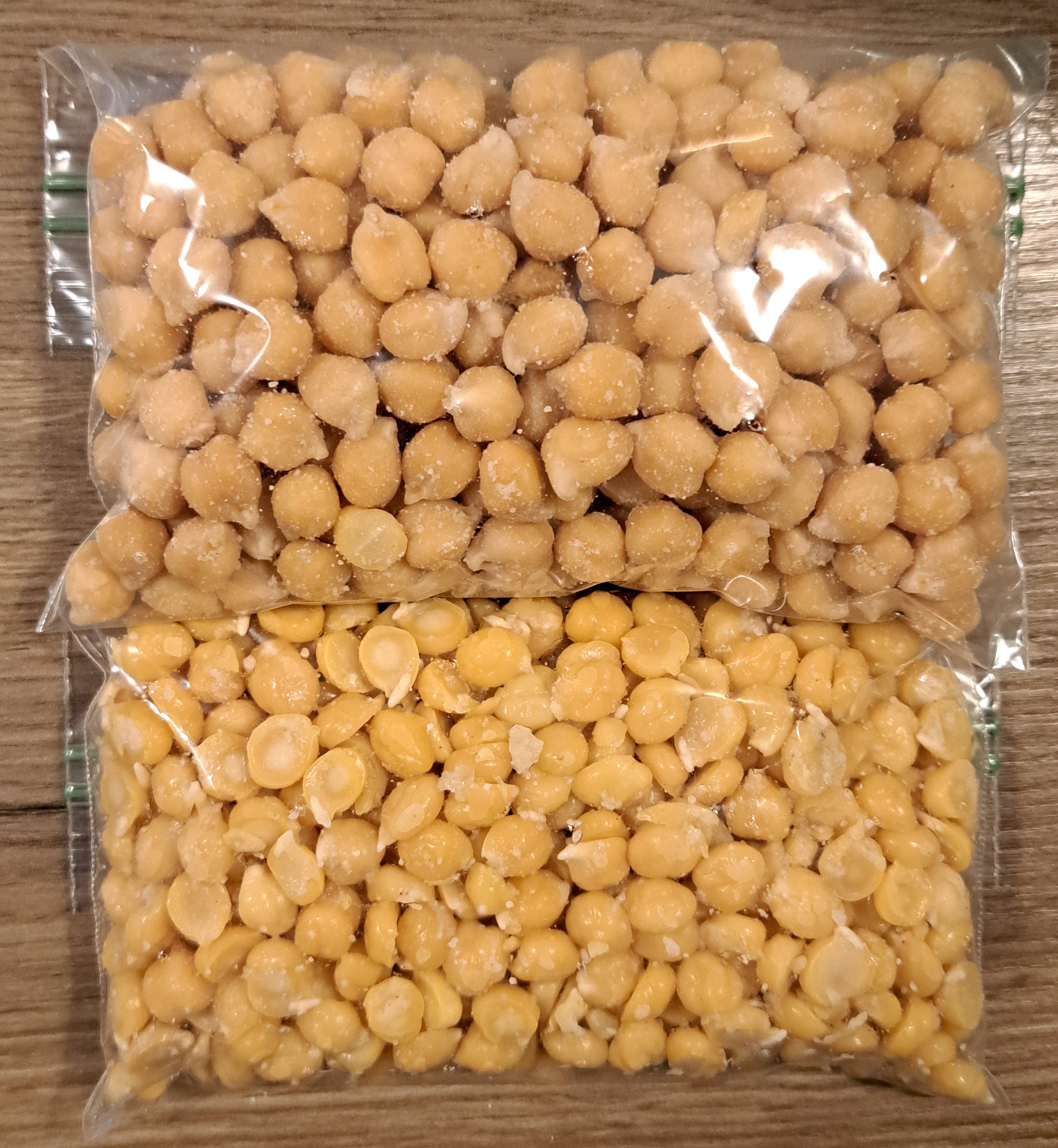
    labels=["No Husk, split", "Husk", ], loc="lower center",**graph_style.legend_style, ncols=3)
plt.setp(legend_title.get_title(), **graph_style.legend_title_style)

# Apply graph styles.
ax.set_title(label="Temperature in different Tempehs", **graph_style.title_style)
ax.set_xlabel(xlabel="Time in hours", **graph_style.axes_style)
ax.set_ylabel(ylabel="Temperature in °C", **graph_style.axes_style)
ax.tick_params( **graph_style.tick_style)
ax.set(xlim=(first_time, last_time), ylim=(20, 40));

That would be the data as measured by the temperature sensors. For illustration purposes, let's add some more information.

# Draw horizontal lines at 30°C. This is the incubation temperature.
ax.hlines(y=30, xmin=first_time, xmax=last_time, label="h_line",
    colors=graph_style.colors_pomegranate[0], ls='--', lw=2)

# Add arrow to gap.
ax.annotate("Data gap", xy=(30, 36), xytext=(10, 38), xycoords='data',
    arrowprops=graph_style.arrow_style,
    **graph_style.annot_text_style)

# Add arrow to end of first tempeh.
ax.annotate("Tempeh done", xy=(46, 38.5), xytext=(53, 33), xycoords='data',
    arrowprops=graph_style.arrow_style,
    **graph_style.annot_text_style)

# Redraw the the legend to include the incubator temperature.
handles, labels = ax.get_legend_handles_labels()
legend_title = ax.legend(title=None, handles=handles,
    labels=["No Husk, split", "Husk", "Incubator"], loc="lower center",
    **graph_style.legend_style, ncols=3)
plt.setp(legend_title.get_title(), **graph_style.legend_title_style)

# Show the plot again.
fig

Ok. A few things are noteworthy:

1. One might wonder why the incubator temperature graph does not look as unstable as before. I actually did not monitor the incubator temperature this time, as both of my thermometers were in one tempeh each. But it is set to 30 °C, so that is what the dashed line shows.
2. There is a rift in the most interesting part of the graphs! My sensors failed at some point. Luckily, I found a way to prevent this issue in the future by reprogramming the data collection process.
3. The graph for the tempeh with the processed chickpeas drops, because after less than 50 hours this tempeh looked done. I took the thermometer out and saved this tempeh, while I gave the other one more time.

The main takeaway, of course, is that the tempeh from peeled and split chickpeas becomes hotter faster than the tempeh from unprocessed peas. More metabolic heat translates to faster growth. Does that mean that the fungus cannot break down the husk? It can at least not utilize it as well as the rest of the peas for its own growth. If we look at the two tempehs after circa 2 days for fermentation, we can see that the one from peeled and split chickpeas looks perfectly done, while the other one looks rather unattractive. It needed another day, and even then, it did not look as nice as the processed tempeh.

Conclusion

Chickpeas should be peeled and split for tempeh production.
I can definitely recommend this after having done many more fermentations with both processed and unprocessed chickpeas.